Django employee website 2
Now the next step is to customise the login page. I want to use the template for the homepage for the login page. As right now it looks like this:
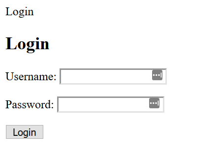
A plain page without CSS. So we need to extend to template to page. When we add the extending tag to the login HTML we get this:

So the template of the website shows up but not the username and login. Later on, I found a somewhat fix by change by changing the {% block content %} tag with an {% block body %}. But as we can see the below the login title is blocked by the header in the way. So we need it so the text can be visible.

Was able to find a fix by designing the template based on the flask tutorial earlier. So I added some div class and line breaks.

Testing in the logging again, get the page stuck on the loading section

But when I manually changed into the home it is logged in.

Not to sure what is the problem with redirecting.
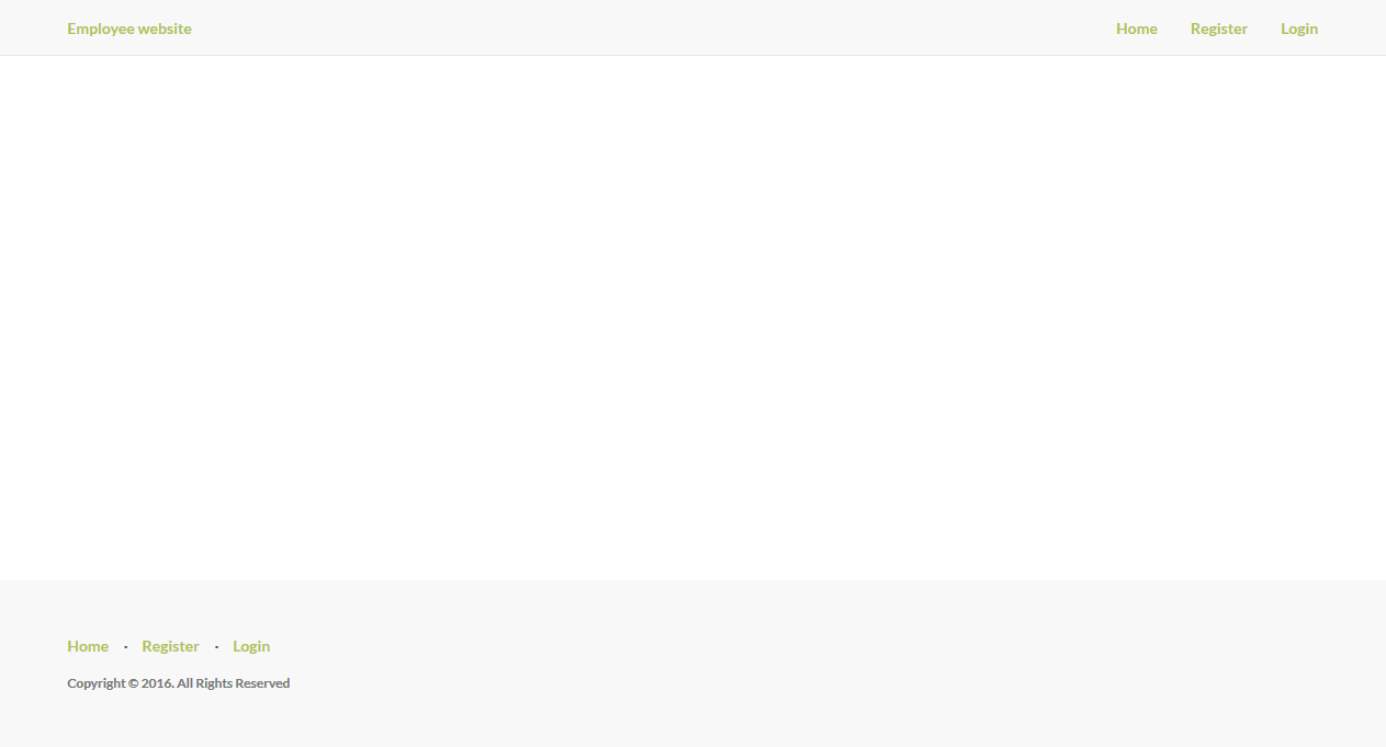
Now we should change the navigation bar links now that I’ve logged in with test employee. We need to have based if the user is logged in so menu options changes. Instead of keeping the menu of register, login and home.
Also the footer below:
Now we have this result when logged in:


Now but the links of the page are still dead so they need to be changed. As the homepage is already in the url.py file it should be simply link to add. And the logout page will be part of the built-in authentication views.
Now we have added the links we test them out. First is the logout link, when clicking it we get this:

I didn’t know why it redirects me into Django admin page, when first tested it. I later found out that it gives the admin page as it doesn’t have a redirect URL to route to. So I need setup a LOGOUT_REDIRECT_URL variable in the app settings to fix the problem. I choose the same option as the login page as it will route to the homepage.
LOGOUT_REDIRECT_URL = '/employee_web'
By logging again we are also testing the login link as well. I was able to get to the login page and login to the website. Now to login back out again to see if redirects to another page.
This page when logged:

When logged out:

The redirect URL changes works as we can see. As this text used from the flask tutorial, I’m basing this website on. The profile link is left dead because I needed to create a template for it with other features. And were only testing the links.
Now to start the building the profile page. The idea of the page is to display information about the user. Email, name. department role etc. First, I’m going to keep the page simple like so:
{% extends "employee_web/base.html" %}


{{ user.username }}
{{ user.email }}
{{ user.first_name }}
{{ user.last_name }}
The next thing I need to do adds to the views and URLs file as this is a new page. And this is not using built-in views or URLs, unlike the authentication views.
The profile view:
def profile(request):
    return render(request, 'employee_web/profile')
And the URLs file:
from django.urls import path

from . import views

urlpatterns = [
    path('', views.home, name='home')
    path('profile', views.profile, name='profile')
]
When trying to test it got this error:

As we can see it can not find the template. Later found the issue which was a simple of mistake of not adding a .html to the end of the template name in the view file. Like so:
def profile(request):
return render(request, 'employee_web/profile.html')
After I loaded the page I got this:

But the problem is similar to the login page issue from earlier. So I just added content block tag. Also has the same out place text issue from earlier:

Which should be fixed with the centre tag and content section. Now the issue is fixed:

But the page is not displaying all the details. Only the username. To make it clearer I added more details to the page to highlight the issue

I think the issue is that in the template I’m accessing the User model not the employee model were all the data is. So I will change the tags in the template to the employee objects. When testing this out it did not work:

And the code:
<h1>Profile</h1>
           <h1>Profile</h1>
            username: {{ Employee.username }} <br>
            email: {{ Employee.email }}<br>
            first_name: {{ Employee.first_name }} <br>
            secord_name: {{ Employee.last_name }} <br>
            role: {{Employee.role}} <br>
            department: {{Employee.department}} <br>
I decided to add names to the User model to see if it would appear in website

So needed to edit the HTML again to display the User model variable. Testing it again it did not work:

I may fix this issue later on as I couldn’t find the fix for problem. I will end the article on this almost complete website.
Django employee website
This project is about creating software that can be used in an enterprise context. So I settled on an employee management system. Mainly an internal website used by the company. This has been done before I will be using this article an inspiration. I will probably use Django instead as the library has more built-in resources for making a tool like this. Useful features such as password management and built-in admin page. I want to make the app with a workable database and website. Not sure if I will deploy the website. If I do deploy I will google cloud services as I have experience with that product or try amazon web services.
First thing is to start creating the database. This is done in Django by making models. From the Django documentation, it defines models as ‘A model is the single, definitive source of information about your data.’ We need to make an model for the employee. The class will the features of first names, last names, id numbers (Django does this automatically), departments and roles.
I briefly forgot I had make an Django app not just use the admin folder given to me. But a simple python manage.py startapp employee_web created the app with an models.py file. So just pasted code for the employee class there.
Now I just to migrate it, using python manage.py migrate. This installs the databases necessary for the installed apps in the settings. The installed apps are these
django.contrib.admin – The admin site. You’ll use it shortly.
django.contrib.auth – An authentication system.
django.contrib.contenttypes – A framework for content types.
django.contrib.sessions – A session framework.
django.contrib.messages – A messaging framework.
django.contrib.staticfiles – A framework for managing static files.
https://docs.djangoproject.com/en/3.0/intro/tutorial02/

Now with python manage.py makemigrations employee_web we can update the employee model to Django.

Now the next step is to set up the admin website. Where we can add users, departments, etc.
python manage.py createsuperuser creates an admin for us.
Email address: admin@example.com
Password:
Password (again):
This password is too common.
Bypass password validation and create user anyway? [y/N]: y
Superuser created successfully.
After logging in you get to see the admin website:

To see the employee model I’ve made earlier, I needed to do the admin.py file and import the employee model

When I click the add employee button it gives me this page:

Which are the fields that I coded in the model earlier. Which means we are making good progress.
Now the next step is to step the views for the website. I going to have a homepage view that will work as a placeholder. The page will have an image in the middle with text over it. Also, have an navigation bar for the employee’s status.
It will be based on this:

Using the code from the tutorial above to develop the page. So I created a folder to hold the HTML file. Pasted the code like so:

Made a simple view function in a new view.py file. So the template can be rendered by Django.
Then next step is to add the view to the urls.py file of the employee_web app.
After then add the path to my employee_site url config.
path('employee_web/', include('employee_web.urls'))

This means I need to delete some of the code on the HTML as it’s not suited to Django parsing. I was able to fix the issue by deleting links that did not link any file or page. And turning other links into dead links so it does not crash the website.
Stuff like this: <li><a href="{ }">Home</a></li>
As we can see the navigation bar loads but not the rest. So my task is not make sure an image is able show on the website. To do this I need to set up an CSS file and folder to host the image. I will the CSS from the same tutorial from earlier.

But some edits need to be made as it was originally designed in flask in mind.
background: url(../img/intro-bg.jpg) no-repeat center center;
will be replaced with:
background: url("images/photo-of-people-sitting-beside-table-3182755.jpg") no-repeat center center;
Also, I will need to add a link to the HTML file so it can get the CSS code.
<link rel="stylesheet" href="{% static 'employee_web/style.css' %}" type="text/css">
Later I found I needed to make a subdirectory to hold the images, so did like so:

Now running the server the again I get this result:
This means it has loads all loads CSS correctly expect the image.
To fix this issue I’m going to make a base HTML template rather using just the one file for homepage. From doing this I fixed the issue:

From looking at the code I noticed that the image that was in the CSS file was under a class that was not in the original homepage file.

Finding the element in the original homepage file:

I think I’ve should have followed the tutorial more closely rather than customising straight away.
Logging in
Now we have a working homepage page. We can start to develop an way for the employee can login into the website. So I have to develop a login page for this. From googling around I’ve found out that Django provides built-in views that handle authentication like login forms. To add the forms to the project just needed to add the views to my URLs file.
I made an folder under my templates called registration which will hold the login html file. I will using the code from this website for the login page. This is the result below:

Now we need to redirect user to the homepage when they can successfully logged in.
From lots of reading I’ve notice I made a major I mistake when making the models. Instead of creating an custom model eg employee. I’ve should have used Django built-in user model. As this is the model being used for the authentication.
To fix this I need to way to connect the employee model to an user class. To do so need to add a one to one field.
user = models.OneToOneField(User, on_delete=models.CASCADE)
The prompt gave an error about adding a new filid but his can be fixed by adding null=true to the user variable.
I added a non-admin user to test this stuff out. This is the employee object below:

Which means this test user has an login. So the user can be redirect into the homepage after logging in I need to change the LOGIN_REDIRECT_URL as the default is /accounts/profile/. I changed into LOGIN_REDIRECT_URL = '/employee_web' which is the route of the homepage. (This will be changed later into something home, to make it more clearer.)
In the homepage I added a if statement to write an message on the website if they logged on.

In the next version should add more features like customising login page. Having an register page etc.
Machine learning and GANs part 2
The first part was going through the code that dealt with the processing of the images and importing the packages for the program. Now this part is going through the shape of the network itself.
The TF_GAN tutorial starts defining functions for the layers.
def _dense(inputs, units, l2_weight):
  return tf.layers.dense(
      inputs, units, None,
      kernel_initializer=tf.keras.initializers.glorot_uniform,
      kernel_regularizer=tf.keras.regularizers.l2(l=l2_weight),
      bias_regularizer=tf.keras.regularizers.l2(l=l2_weight))
As we can see this creates the dense layer. The arguments for the function are inputs, units, l2 weight. The inputs are the image data being put through the network. Units which are another word neuron for the network. L2_weights stands for layer 2 weights. Weights are the measure are how strong a connection is to another neuron.
kernel_initializer is are ways to start with random weights for your model.
kernel_regularizer reduces overfitting by adding penalties to the weights
bias_regularizer which tries to reduce the bias of network
def _batch_norm(inputs, is_training):
  return tf.layers.batch_normalization(
      inputs, momentum=0.999, epsilon=0.001, training=is_training)
This is the batch normalisation layer. Batch normalisation is a technique which normalises output from layers within the neural network.
def _deconv2d(inputs, filters, kernel_size, stride, l2_weight):
  return tf.layers.conv2d_transpose(
      inputs, filters, [kernel_size, kernel_size], strides=[stride, stride],
      activation=tf.nn.relu, padding='same',
      kernel_initializer=tf.keras.initializers.glorot_uniform,
      kernel_regularizer=tf.keras.regularizers.l2(l=l2_weight),
      bias_regularizer=tf.keras.regularizers.l2(l=l2_weight))
This layer is a Deconvolution layer or an Transposed convolution layer. These layers are part of Convolutional Neural Networks. Networks like those can scan an image and learn different features of the images. Which can be used to difference between the images.
The arguments of the function are simply settings for the how the deconvolutional layer will scan the image. Most of them can be found here.
Filters argument size of which filters/scans through the image.
Kernel_size is the size the convolution window. The convolution window also known as the kernel.
Strides is the movement of the kernel along the image.
The next returns a Conv2DTranspose class. Which is a TensorFlow layer. The class uses the same arguments defined from the earlier function. The kernel size and the strides used a list of two integers.
activation=tf.nn.relu, padding='same',
This line defines the activation function. Padding
kernel_initializer=tf.keras.initializers.glorot_uniform,
      kernel_regularizer=tf.keras.regularizers.l2(l=l2_weight),
      bias_regularizer=tf.keras.regularizers.l2(l=l2_weight)
these lines are the same as in the dense layer.
def _conv2d(inputs, filters, kernel_size, stride, l2_weight):
  return tf.layers.conv2d(
      inputs, filters, [kernel_size, kernel_size], strides=[stride, stride],
      activation=None, padding='same',
      kernel_initializer=tf.keras.initializers.glorot_uniform,
      kernel_regularizer=tf.keras.regularizers.l2(l=l2_weight),
      bias_regularizer=tf.keras.regularizers.l2(l=l2_weight))
The tf.layers.conv2d details are the same as the _deconv2d layer. But there is no activation function.

Using the layers, the tutorial just defined earlier. The next is the develop an generator. The first line
is_training = (mode == tf.estimator.ModeKeys.TRAIN)
Sets the generator to make sure its one training mode.
net = _dense(noise, 1024, weight_decay)
net = _batch_norm(net, is_training)
net = tf.nn.relu(net)
The net variable stacks on layers on top of each other. The first layer is the dense layer as noise as the input and 1024 units. And weight decay from the generator argument above. The next layer is an batch normalisation with net variable as the input argument and the training argument set to is_traisning. Third line is an tensorflow activation function relu. With the prevois layer out though it.
net = _dense(net, 7 * 7 * 256, weight_decay)
net = _batch_norm(net, is_training)
net = tf.nn.relu(net)
The next layers added to the neural network is an other dense layer. The previous layers as the input. 7 * 7 * 256 as the units. The next line is another batch norm like before. The next layer is an other relu activation function.
net = tf.reshape(net, [-1, 7, 7, 256])
net = _deconv2d(net, 64, 4, 2, weight_decay)
net = _deconv2d(net, 64, 4, 2, weight_decay)
# Make sure that generator output is in the same range as `inputs`
# ie [-1, 1].
net = _conv2d(net, 1, 4, 1, 0.0)
net = tf.tanh(net)
net = tf.reshape(net, [-1, 7, 7, 256])
Changes the shape of the of the tensor input from the previous layer of the network.
net = _deconv2d(net, 64, 4, 2, weight_decay)
net = _deconv2d(net, 64, 4, 2, weight_decay)
Two deconv2d layers are added with the previous layers as inputs. 64 filters. 2 as the number for kernel size.
net = _conv2d(net, 1, 4, 1, 0.0)
net = tf.tanh(net)
A convonultal layer with 1 filter, 4 as the kernel size, 1 equaling to stride and 0.0 equaling layer 2 weight.
Ending with an tanh activation layer.
At the end the function it returns the generator as the net variable.

First the tutorial defines an leaky relu. Another type of activation function.
Defining the discriminator the first line in the function is to delete unused conditioning. The next line sets up the training mode.
Like the generator it stacks layers using the net variable. The first layer is a convolution layer. With the image as the input. 64 filters, 4 as kernel size, 2 as strides.
After that an activation function of the leaky relu is added.
The next convolutional layer is the same, except from the filter which is now 128. Another leaky relu layer is added.
The next layer flattens the inputs from coming from previous layers.
After that the new dense layer is added with 1024 units. An batch norm layer is added with training mode set on. And another leakly relu is added.
The final layer is an dense layer with 1 unit.
The return statement gives the layers produced in variable form.

Now the tutorial has section for evaluating the model.
from tensorflow_gan.examples.mnist import util as eval_util
The tutorial imports the ulties for evaluating models.
real_data_logits = tf.reduce_mean(gan_model.discriminator_real_outputs)
gen_data_logits = tf.reduce_mean(gan_model.discriminator_gen_outputs)
defines the logits of the discromator and generator.
real_mnist_score = eval_util.mnist_score(gan_model.real_data)
generated_mnist_score = eval_util.mnist_score(gan_model.generated_data)
frechet_distance = eval_util.mnist_frechet_distance(
gan_model.real_data, gan_model.generated_data)
This works out scores of the mist data. Using the tensorflow_gan.examples.mnist util package to help evaluate the scores
return {
'real_data_logits': tf.metrics.mean(real_data_logits),
'gen_data_logits': tf.metrics.mean(gen_data_logits),
'real_mnist_score': tf.metrics.mean(real_mnist_score),
'mnist_score': tf.metrics.mean(generated_mnist_score),
'frechet_distance': tf.metrics.mean(frechet_distance),
}
This code block returns the stats of the scores calculated.

train_batch_size = 32 #@param
noise_dimensions = 64 #@param
generator_lr = 0.001 #@param
discriminator_lr = 0.0002 #@param
These blocks set up the parameters for the model. The Constructor helps piece together the GAN model. This called the GANEstimator.
def gen_opt():
gstep = tf.train.get_or_create_global_s tep()
base_lr = generator_lr
# Halve the learning rate at 1000 steps.
lr = tf.cond(gstep < 1000, lambda: base_lr, lambda: base_lr / 2.0)
return tf.train.AdamOptimizer(lr, 0.5)
This function helps optimise the generator more by decreasing the learning rate.
gstep = tf.train.get_or_create_global_s tep()
The global step rate for the model.
base_lr = generator_lr
Creating a variable which the base learning rate will match the generator learning rate.
gan_estimator = tfgan.estimator.GANEstimator(
generator_fn=unconditional_generator,
discriminator_fn=unconditional_discriminator,
generator_loss_fn=tfgan.losses.wasserstein_generator_loss,
discriminator_loss_fn=tfgan.losses.wasserstein_discriminator_loss,
params={'batch_size': train_batch_size, 'noise_dims': noise_dimensions},
generator_optimizer=gen_opt,
discriminator_optimizer=tf.train.AdamOptimizer(discriminator_lr, 0.5),
get_eval_metric_ops_fn=get_eval_metric_ops_fn)
This the gan estimator constructer:
generator_fn=unconditional_generator,
discriminator_fn=unconditional_discriminator,
These variables define the generator and discriminator functions using the functions made earlier.
generator_loss_fn=tfgan.losses.wasserstein_generator_loss,
discriminator_loss_fn=tfgan.losses.wasserstein_discriminator_loss,
These define the loss functions for generator and the discriminator. The loss function Wasserstein los function. This loss function tends to make the model more stable. As the loss rate less likely to fluctuate and stay stuck.
params={'batch_size': train_batch_size, 'noise_dims': noise_dimensions},
Sets the parameters set from earlier in a dictionary.
generator_optimizer=gen_opt,
discriminator_optimizer=tf.train.AdamOptimizer(discriminator_lr, 0.5),
get_eval_metric_ops_fn=get_eval_metric_ops_fn)
Sets up optimisers and collects metrics.

The tutorial’s comments does a good job the code.
tf.autograph.set_verbosity disables extra text from the output when training.
import time
steps_per_eval = 500 #@param
max_train_steps = 5000 #@param
batches_for_eval_metrics = 100 #@param
More parameters set up which we can use the custom text options to the right to change the pararmeters.
steps = []
real_logits, fake_logits = [], []
real_mnist_scores, mnist_scores, frechet_distances = [], [], []
Like the comment said the list is used to track metrics.

Cur_step is the variable for current step which is step to 0.
start_time = time.time()
Start time defined my the current when the program got this point.
while cur_step < max_train_steps:
next_step = min(cur_step + steps_per_eval, max_train_steps)
While loop that states that if the max training step is larger then the current step then continue.
next_step is done by adding the current step and step per evaluation compared to the max training steps.
start = time.time()
gan_estimator.train(input_fn, max_steps=next_step)
steps_taken = next_step - cur_step
time_taken = time.time() - start
print('Time since start: %.2f min' % ((time.time() - start_time) / 60.0))
print('Trained from step %i to %i in %.2f steps / sec' % (
cur_step, next_step, steps_taken / time_taken))
cur_step = next_step
Like the tutorial said in the text description of this section. It repeatedly calls train function gan estimator to show the genitor output. Start equals time the line of code is run.
gan_estimator.train(input_fn, max_steps=next_step)
input function used to feed in data and max_step is set to the next step.
steps_taken = next_step - cur_step
time_taken = time.time() – start
The step taken is worked out by the difference next_step and current step. time_taken worked out by difference between the start and current time.
print('Time since start: %.2f min' % ((time.time() - start_time) / 60.0))
print('Trained from step %i to %i in %.2f steps / sec' % (
cur_step, next_step, steps_taken / time_taken))
cur_step = next_step
These print statements print out time of training and step. With formatting.
metrics = gan_estimator.evaluate(input_fn, steps=batches_for_eval_metrics)
steps.append(cur_step)
real_logits.append(metrics['real_data_logits'])
fake_logits.append(metrics['gen_data_logits'])
real_mnist_scores.append(metrics['real_mnist_score'])
mnist_scores.append(metrics['mnist_score'])
frechet_distances.append(metrics['frechet_distance'])
print('Average discriminator output on Real: %.2f Fake: %.2f' % (
real_logits[-1], fake_logits[-1]))
print('Inception Score: %.2f / %.2f Frechet Distance: %.2f' % (
mnist_scores[-1], real_mnist_scores[-1], frechet_distances[-1]))
This block is mainly to calculate metrics.
metrics = gan_estimator.evaluate(input_fn, steps=batches_for_eval_metrics)
Gets the first evaluate from the input function and the batches for evaluation.
steps.append(cur_step)
real_logits.append(metrics['real_data_logits'])
fake_logits.append(metrics['gen_data_logits'])
real_mnist_scores.append(metrics['real_mnist_score'])
mnist_scores.append(metrics['mnist_score'])
frechet_distances.append(metrics['frechet_distance'])
These lines of code simply append the data into lists.
print('Average discriminator output on Real: %.2f Fake: %.2f' % (
real_logits[-1], fake_logits[-1]))
print('Inception Score: %.2f / %.2f Frechet Distance: %.2f' % (
mnist_scores[-1], real_mnist_scores[-1], frechet_distances[-1]))
These print statements output the scores of the training.
# Vizualize some images.
iterator = gan_estimator.predict(
input_fn, hooks=[tf.train.StopAtStepHook(num_steps=21)])
try:
imgs = np.array([next(iterator) for _ in range(20)])
except StopIteration:
pass
tiled = tfgan.eval.python_image_grid(imgs, grid_shape=(2, 10))
plt.axis('off')
plt.imshow(np.squeeze(tiled))
plt.show()
this block of code shows some of the image.
iterator = gan_estimator.predict(
input_fn, hooks=[tf.train.StopAtStepHook(num_steps=21)])
try:
imgs = np.array([next(iterator) for _ in range(20)])
except StopIteration:
pass
Try excpect block creates an variable for the images by iterating though iterator variable.
tiled = tfgan.eval.python_image_grid(imgs, grid_shape=(2, 10))
plt.axis('off')
plt.imshow(np.squeeze(tiled))
plt.show()
Turns the images into grid form
# Plot the metrics vs step.
plt.title('MNIST Frechet distance per step')
plt.plot(steps, frechet_distances)
plt.figure()
plt.title('MNIST Score per step')
plt.plot(steps, mnist_scores)
plt.plot(steps, real_mnist_scores)
plt.show()
Adds the steps and metrics close to the images.
Machine Learning and GANs Part 1
Today I will be trying to teach myself how to develop GANs. Which stand for Generative adversarial networks. This is a machine learning model which contains a “Generative” model and a “Discriminative”. The Generative model generates data and the Discriminative model which inspects the different type of data shown to it.
I have some previous experience playing around with machine learning, so this project should act as a refresher. I will be using Google’s machine learning course.
The structure of a GAN contains the generator which create fake data which later to be used in with the discriminator which tries to spot the different between the fake data. When the discriminator detects the data given to it is fake it punishes the generator. This allows the generator to get feedback and get better. If the discriminator incorrectly guesses the fake data is real it will get punished and also collect feedback and get better.

Training
The generator and discriminator has different training method. So they cant be run at the same time. So the GAN must alternate between the discriminator and the generator. As the later generator later improves the discriminator’s performance decreases because the discriminator struggles to see the different between fake or real data.
Coding up the example
Using the Google TF Gan Package. Read though the example to see how an GAN is developed line by line.

import tensorflow_gan as tfgan
This line of code imports the tensorflow GAN package. This is an library which makes it easier to train and analyse GANs.
import tensorflow_datasets as tfds
This line imports the tensorflow datasets. These are normally used for example projects. As in real life projects you be using your own data.
import matplotlib.pyplot as plt
This line is used to show images of the data. This so we can actually see the data.
import numpy as np
This is done to multiplate the arrays and matrices in the code. To change the shape of the array etc.

assert 'batch_size' in params
assert 'noise_dims' in params
The assert statements are used to use if an condition is true. These assert statements are testing to see if the variables('batch_size' and 'noise_dims') are in the correct parameters.
bs = params['batch_size']
nd = params['noise_dims']
These assigns variables to the parameter keys of the batch size and noise dimensions. The reason why it’s a key is because the params are set up in a dictionary later on.
split = 'train' if mode == tf.estimator.ModeKeys.TRAIN else 'test'
shuffle = (mode == tf.estimator.ModeKeys.TRAIN)
just_noise = (mode == tf.estimator.ModeKeys.PREDICT)
These variables set up mode argument for the function. The first line sets to training mode which is saved in the split variable. Which is used to split the dataset form training and prediction. The second line sets the function to training mode as well. If the argument is set to shuffle. This variable is used in an if statement later on. The third variable sets the mode to prediction mode if just noise is set.
noise_ds = (tf.data.Dataset.from_tensors(0).repeat()
              .map(lambda _: tf.random_normal([bs, nd])))
This line of code produces random noise sample. tf.data.Dataset.from_tensors(0) creates an dataset object. The repeat function repeats the dataset an infinite number of times. The map function transforms the tensors with random numbers in the shape of the batch size and noise dimensions.

This new function pre-processes images. The first line is explained with the comment, that the code maps the image of a shape of 0, 255 to -1, 1. The reason why the these numbers are chosen is because 255 is the bytes of the image. The -1 and 1 is the converting to a float data type.
images = (tf.cast(element['image'], tf.float32) - 127.5) / 127.5(tf.cast(element['image'], tf.float32)
Tf.cast coverts tensor to a different data type. Inside the tf cast function is the element parameter of the pre-process function and tf.float32. So the image is converted into a float32 datatype.
- 127.5) / 127.5
This normalises the data. Normalisation data preparation techniques used to change number based columns to an common scale. And the pixels of the images scaled into an -1 and 1 shape.
images_ds = (tfds.load('mnist', split=split)
               .map(_preprocess)
               .cache()
               .repeat())
The images_ds variable main job is to load the mnist dataset. The tfds.load function loads the named dataset into the program. The named dataset is the MNIST dataset. The function uses a spilt argument which is set the split variable from earlier.
.cache() function caches the elements
.repeat() repeats the functions that ran earlier.
if shuffle:
    images_ds = images_ds.shuffle(
        buffer_size=10000, reshuffle_each_iteration=True)
  images_ds = (images_ds.batch(bs, drop_remainder=True)
               .prefetch(tf.data.experimental.AUTOTUNE))
The if statement is added if the shuffle option is picked.
The .shuffle() function randomly shuffles the items in the dataset. The buffer_size argument decides how large buffer would be. The buffer is a selection of elements in the dataset. The shuffle function would select randomly from the buffer selection with chosen elements replaced with new ones.
reshuffle_each_iteration argument means after each iteration it will get reshuffled.
The .batch(bs, drop_remainder=True). This function merges the elements into batches. Using the bs variable from earlier to set the number of the batch size. The drop remainder argument is true to stop a smaller batch sizes being produced if the number of elements is not even.
.prefetch(tf.data.experimental.AUTOTUNE))Creates a Dataset that prefetches elements from this dataset. This is done so training data can be done faster as next item will be ready.
For more infomation check this link
return tf.data.Dataset.zip((noise_ds, images_ds))This line of code zips the datasets of noise and images.

params = {'batch_size': 100, 'noise_dims':64}The parameters are set using the dictionary of the batch size and noise dims.
with tf.Graph().as_default():
This line creates the computation graph were the operations of TensorFlow can run.
ds = input_fn(tf.estimator.ModeKeys.TRAIN, params)
this dataset variable uses the input function from earlier. The mode key is set to train and the parameters set using the params variable from earlier.
numpy_imgs = next(tfds.as_numpy(ds))[1]
This line converts the images into numpy arrays. The next() function is used return next item in the dataset. As_numpy creates a dataset in the numpy format.
img_grid = tfgan.eval.python_image_grid(numpy_imgs, grid_shape=(10, 10))
This line of code allows the images to be shown in an grid which is sotred in a variable
Removes the matplotlib axis when showing the image.

```plt.imshow(np.squeeze(img_grid))
Not too sure will add later.
plt.show()
displays the image.
Reading KML files from google maps
This project should be relatively short. The goal is to make sight edits to a KML file from google maps. A KML is a file used to display information of google maps or google maps. Geolocations, directions etc.
The file I’m using looks like this:

This file consists of outdoor locations around London. To export the file from must choose the “Export KML/KMZ” like below:

Then choose the KML option:

Now we have the file in are project folder we must get the third-party package that will parse through the file.
Using this package called FastKML installed via pip. Reading the docs we can turn the file into a string so it can be read.
The code I used below:
from fastkml import kml

with open('Outdoor London.kml', 'rt', encoding="utf-8") as myfile:
    doc = myfile.read()

print(doc)
The file printed on the command line below:

Now we have the file parse we want to start editing. I want to edit the current icon and also create a new icon with its own location.
So first to edit the current icons we need to scroll down to were the names of the place markers are shown:

In this example, I will shorten the of the place marker to meanwhile Gardens.

Simply done by deleting the text:

Now we want to add a new place marker into the file. Likely I will make a placemark tag with other children tags like above.
Copying and pasting this example to use:

Now I must choose custom coordinates of the location. Using google maps picked a location to decide on:

When adding the coordinates to the file, is that the order of the numbers when copying is the wrong way around. So when paste you must change the order.

Now, with the edited code, we should open the file on google maps
To do that we head to google maps them navigate to your places tabs:

After that we click on the maps tabs then we head to “create new map”:

After we get moved into a new page called google myMaps. Now we can import are KML file:

After uploading the loading the file, we can see the map. Below we can we the custom example I added:

Also, the example edited the text is also changed:

Now we have successfully edited the KML file. From coding this project while writing I noticed that if your KML file does not have much data points then the fastKML library is not needed as you can just directly edit the KML file itself.
Graphs with flask
This project we be me trying to graph some of google sheets data in into a flask website. Using this website to guide me. The spreadsheet I will be trying to graph on the flask website is this:

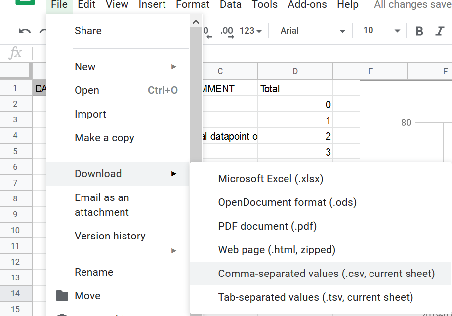
This is a graph of the amount of strangers I’ve tried to talk to in a given amount of time. To have the file in ready for are python program we need to export the spreadsheet into an csv file.
Create an new environment or activate an old where you can have the flask package.
Conda install flask
Pip install flask
After that make an templates folder for the html and app.py to run the data.

The tutorial from above hard-coded the data in the app.py file but as we getting are data from a csv file it will have to be done a little bit differently.
So, we can dealing with the columns more easier I decided to import pandas.
Simple df.head() statement below:

Now we need to separate the columns into list and save it as a variable so we can use them on are graphs. The comment column is not useful so we can drop that.
To turn the columns into list run this code below:
Now the printed results of the first 10 values:
Dates = df['DAYSTAMP'].tolist()

Values = df['Values'].tolist()

Totals = df['Total'].tolist()
Now we the data needed for are program, now we can start coding the flask section of the file.
We going to borrow some the code from the tutorial for writing the app routes and template function.
@app.route('/bar')
def bar():
    bar_labels = Dates
    bar_values = Values
    return render_template('bar_chart.html', title='Convo bar', max=17000, labels=bar_labels, values=bar_values)

@app.route('/line')
def line():
    line_labels = Dates
    line_values = Values
    return render_template('line_chart.html', title='Covo Line', max=17000, labels=line_labels, values=line_values)

@app.route('/pie')
def pie():
    pie_labels = Dates
    pie_values = Values
    return render_template('pie_chart.html', title='Convo Line', max=17000, set=zip(Values, Dates, colors))
Also we need to make the html files to render the template. These were borrowed from the tutorial again.

The graphs does not load correctly as we can see below:

The bar graph has the same issue:

The issue I found is that the max variable which sets the highest number for the y axis is 1700. This makes the numbers in the close to zero as they are now where close to 1700.

I will change it to max 100. The results are below:

As we can see the change did work. But the issue is now formatting issues. As the dates on the x axis are stuffed into each other looking a bit messy. From googling around you need to add maxTicksLimit to the graphs options. But from testing it does not work so decided make my own custom template based on the chart JS usage example.
But I struggled with fixing this problem so an article in later date my be released.
Google map ISS part 4
Now I want to publish the project on the web. For deployment, I decided with google cloud services as this is the deployment systems I’ve used in previous projects.
I will follow the tutorial from their website
First I had to create a new project this was done via the google could website as it was clear how to name the project correctly as the SDK was giving me this:
ERROR: (gcloud.projects.create) argument PROJECT_ID: Bad value [ISS_Google_maps]: Project IDs must start with a lowercase letter and can have lowercase ASCII letters, digits or hyphens. Project IDs must be between 6 and 30 characters.
Usage: gcloud projects create [PROJECT_ID] [optional flags]
  optional flags may be  --enable-cloud-apis | --folder | --help | --labels |
                         --name | --organization | --set-as-default
After we need to run this statement ‘gcloud app create’. This statement activates the google app engine. This is the google cloud product we will use create our web app.Then we need to authenticate ourselves so we can allow local testing.
We do this using this statement:
gcloud auth application-default loginAfterwards we can now start structuring the files for the web-app. According to the website we need to structure a project like this:
building-an-app/
app.yaml
main.py
requirements.txt
static/
script.js
style.css
templates/
index.html
As the JavaScript and CSS code is in the template file itself. I will be skipping making a static folder. I will simply copy the folder where I use for deployment.

The files in the folder:

As we can see we have a lot of useless files, a few leftover files form using google maps plotting packages before I used the custom template from google. For deployment, we don’t need git so that also needs to do.
I need to delete a few imports are not used anymore mainly gmplot package. Also code which is redundant as the package is not needed for the project.
As I've used lots of packages for these projects I will have export them needed packages into a requirements.txt file. As I'm using the Anaconda environment I will use this command below to produce the requirements.txt:
conda list -e > requirements.txtThe result we can see:


Now we have the requirements.txt file completed. We need to test if the deployment version works on the local server. The tutorial says I need to use PowerShell and the virtualenv packages to test the project. So I will not be using my Anaconda environment.
Later I found that you need to use pip freeze > requirements.txt for the requirements.txt file work correctly with pip install. Don’t skip this step.
Now running the app.py in the virtualenv. We get this:

Which means the local server test works.
The tutorial says the step is to set app.yaml file to deploy onto the google servers.
I copied the app.yaml example from the tutorial then modified the code for my project
runtime: python36

handlers:
  # This configures Google App Engine to serve the files in the app's static
  # directory.
# - url: /static
#   static_dir: static

  # This handler routes all requests not caught above to your main app. It is
  # required when static routes are defined, but can be omitted (along with
  # the entire handlers section) when there are no static files defined.
- url: /.*
script: auto
Changed the runtime to python 3.6 as this is the python version I’m using. Commented out the code allowing a static folder as this project does not have one.
Now we are ready to deploy the website to do so we must run this command on the cloud SDK:
gcloud app deployThis was the cloud SDK returned when I pasted the command in. As we can see it is processing project for deployment.

After running this google clould gave me this error:
ERROR: (gcloud.app.deploy) INVALID_ARGUMENT: Invalid runtime 'python36' specified. Accepted runtimes are: [go, php, php55, python27, java, java7, java8, go111, go112, java11, nodejs8, nodejs10, php72, php73, python37, ruby25]
This means I have to the python runtime on python37. Now the command prompt didn’t throw and error

Now to view the web app we must run this command:
gcloud app browseBut loading on my browser web app threw me this error:

After a whole day of googling and debugging. I found the solution is to change the app.yaml file to a flex environment. And have custom entrypoint command. So the file looks like this:
runtime: python
env: flex
entrypoint: gunicorn -b :$PORT app:app


runtime_config:
  python_version: 3


handlers:
  # This configures Google App Engine to serve the files in the app's static
  # directory.
# - url: /static
#   static_dir: static

  # This handler routes all requests not caught above to your main app. It is
  # required when static routes are defined, but can be omitted (along with
  # the entire handlers section) when there are no static files defined.
- url: /.*
script: auto
Before running you need to add gunicorn to requiments.txt so program installs this package which will help the deploy the app to google servers.
I simply added this line at the end of my requiments.txt:
gunicorn==19.9.0
I don’t know most update model or the best for the project but I do know this works.

As we can see the SDK is downloading packages from the requiments.txt file.
This is the SDK after is complete:

Now, this is the website on the google server:

This means the deployment is successful.
If you want to view the website you can the website here:
https://clean-evening-253117.appspot.com
I will probably change the domain to user-friendly and also make sense.
Python ISS Google maps part 3
Now the next steps are to develop the mini-biography sections below the map.
As I’m not an expert on HTML or CSS I did a lot of googling around to find my solution. Where I ended up was using the flexbox feature from CSS. Which responsively changes how the content looks on the page without hard coding how the columns will look like.
This is the result I got:

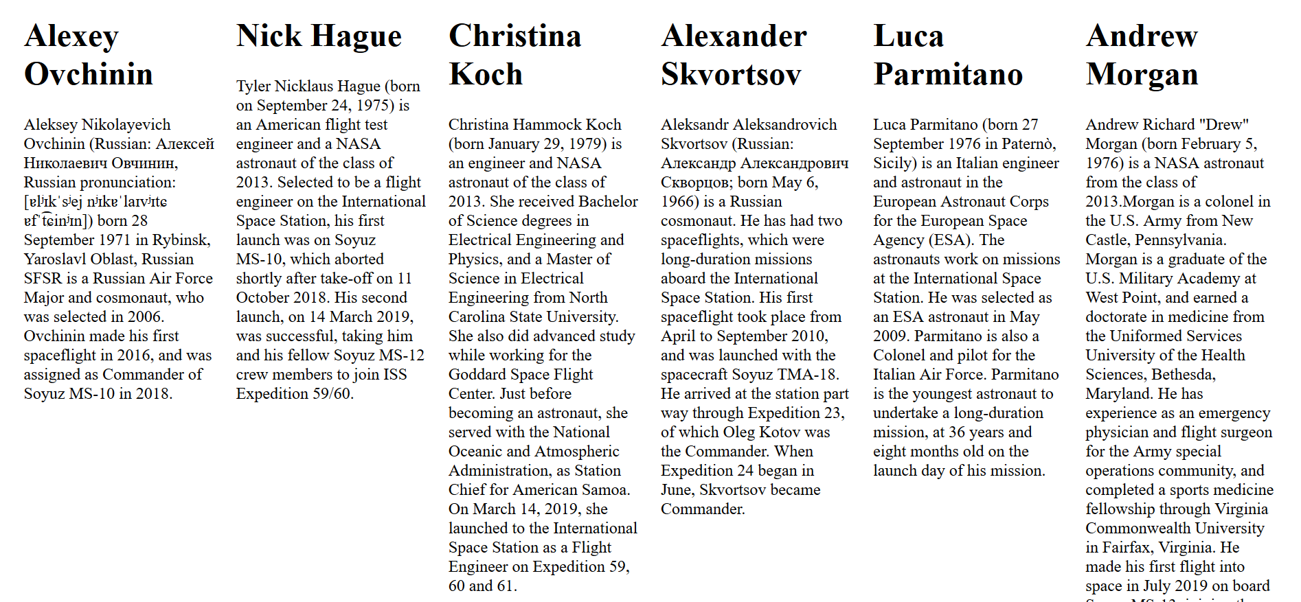
This is the basic structure of how I want bottom half of the page to look. The column headers will be the astronauts' name and the text below is their biographical information from Wikipedia from earlier.
The basic html code is below:
<div class="flex-container">
         <div> <h1>test</h1>Lorem ipsum dolor sit amet,  …..</div>
         <div> <h1>test</h1> Lorem ipsum dolor sit amet,  …..</div>
And CSS:
.flex-container {
        display: flex;
       }
Now we have the basic structure down we need to replace the placeholder texts with flask variables so information from the previous script can be pasted.
To change the column headers I imported the list of astronauts names from the previous script. Then changed the heading text to a variable containing list and the chosen index:
<div> <h1>{{ Names_of_austronuts[0] }}</h1>Lorem ipsum dolor </div>
 <div> <h1>{{ Names_of_austronuts[1] }}</h1> </div>
<div> <h1>{{ Names_of_austronuts[2] }}</h1> </div>
The changes in the web page are shown below:

Now we need to replace the placeholder text below to headers.
Doing something similar, I created list of the Wikipedia summary of the astronauts. The returned the list with a chosen index in the template. Like below:
<div> <h1>{{ Names_of_austronuts[0] }}</h1> {{ desciptions[0] }} </div>
<div> <h1>{{ Names_of_austronuts[1] }}</h1> {{ desciptions[1] }} </div>
<div> <h1>{{ Names_of_austronuts[2] }}</h1> {{ desciptions[2] }} </div>
The results on the web page are below:

Later on, sent a bit more time editing the CSS code so items in flexbox can change to a better size and text to be more aligned.
Current code right now:
flex-container {
        display: flex;
        margin: 5px;

       }
       .item {
         padding:10px;
         flex: 1 1 0px;

       }
Result:
I want to add images of the astronauts on top of the Wikipedia description. Also, I need to link the sections to the Wikipedia page and assign Wikipedia credit on the website.
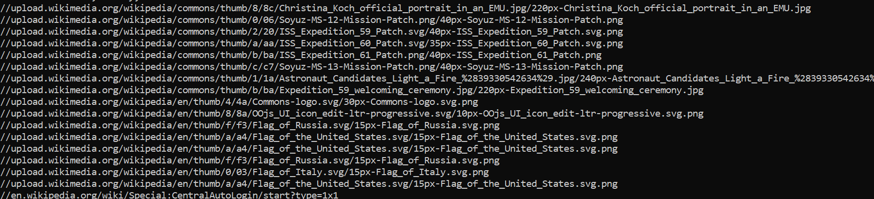
To get images of the astronauts from Wikipedia we need to use the API from earlier to fetch the links. Create a list were links are stored and can be used in the template. To get link we need the API to load the page then select the images.
I append them like this:
links_for_images.append(wikipedia.page(every_person.images[0]))Then added images tags to the template like this:
<img src="{{ Links[0] }}" alt="">
<img src="{{ Links[1] }}" alt="">
<img src="{{ Links[2] }}" alt="">
The result of the images was looked like this:

As we can see the biography section of the website is coming to get her. The main issue is that some of the astronauts don’t have their portrait photo selected, mainly Nick Hague and Christina Koch.
I think I need to design custom solution images are picked from the infobox section. To do so I imported beautifulsoup to make I own custom scraper to scraper scrap the Wikipedia pages.
To get the URLs I used the Wikipedia package to return the links of the searched astronauts and then appended them to a list.
Link_of_page.append(wikipedia.page(every_person).url)After that I used the request library to retrieve the web page via HTTP:
hidden_page_results = requests.get(Link_of_page[2])
page_results = hidden_page_results.content
The .content attribute returns the html from the web so it can be used for the scraper im making.
With that I passed the page_results variable into the beautifulsoup function so the package can parse the code. Afterwards I made a variable containing all the HTML code in the Infocard where the portrait picture is located.
soup = BeautifulSoup(page_results, 'html.parser')
infocard = soup.find('infobox biography vcard')
Now borrowing some of the code I found from this GitHub gist I scraped the links in the infobox.
image_tags = soup.findAll('img')

for image_tag in image_tags:
    print(image_tag.get('src'))
Now, these are the print statements below:
The code above only allowed one link so I will modify the code so it run through all links in the list.
The for loop I came with is this:
for every_link in Link_of_page:
    HTTP_results = requests.get(every_link)
    page_results = HTTP_results.content

    soup = BeautifulSoup(page_results, 'html.parser')
    infocard = soup.find('infobox biography vcard')
    image_tags = soup.findAll('img')

    links_image_tags = []
    for image_tag in image_tags:
        print(image_tag.get('src'))
        links_image_tags.append(image_tag.get('src'))

    links_for_images.append(links_image_tags[0])
The links_image_tags is used so I can receive the first image tag without collect all of the rest.
My results:

As we can see it was able to get most of the portraits but some captured useless images not relevant to the project.
The issue I later found out was I was not extracting the HTML properly. The previous code extracted all the images in the Wikipedia page, not the infobox section. Because of it captured the first image it all on the page similar to the previous code where I used the Wikipedia package to extract the images.
Before:
soup = BeautifulSoup(page_results, 'html.parser')
infocard = soup.find('infobox biography vcard')
image_tags = soup.findAll('img')
After:
soup = BeautifulSoup(page_results, 'html.parser')
infocard = soup.find('table', class_='infobox biography vcard')
image_tags = infocard.findAll('img')
Now running the flask application again I get the website looking like this:

Now all of the astronauts have their portrait showing we can starting styling up the website.
Using the bootstrap library I will the website more appealing. By changing the div tags to bootstrap approved tags like below:
<div class=".container-fluid">
      <div class="row">
        <div class="col border">
        <div class="col border">
        <div class="col border">
The result made the website more presentable see below:

Like I mentioned earlier I wanted to link the profiles of the astronauts to their Wikipedia pages so people can see more information about them. I simply added anchor tags within the header tags and imported the list containing the URLs of the pages.
<h1><a href="{{ Links_pages [0] }}">{  }</a></h1>
<h1><a href="{{ Links_pages [1] }}">{  }</a></h1>
<h1><a href="{{ Links_pages [2] }}">{  }</a></h1>
Also changing the header above the columns, the website looks like this:

The website is basically done. I think more details should be added to the website. Probably some text about where the International Space Station is. Ex the ISS is now in India, Right now it’s located in the Atlantic ocean. As it just shows the GPS location on google maps.
To get the text of where the ISS is located we need to go back where is originally JSON file is produced by the Google maps geocode API.
The Json file looks like this:
[{'address_components': [{'long_name': 'Indian Ocean', 'short_name': 'Indian Ocean', 'types': ['establishment', 'natural_feature']}], 'formatted_address': 'Indian Ocean', 'geometry': {'bounds': {'northeast': {'lat': 10.4186036, 'lng': 146.9166668}, 'southwest': {'lat': -71.4421996, 'lng': 13.0882271}}, 'location': {'lat': -33.137551, 'lng': 81.826172}, 'location_type': 'APPROXIMATE', 'viewport': {'northeast': {'lat': 10.4186036, 'lng': 146.9166668}, 'southwest': {'lat': -71.4421996, 'lng': 13.0882271}}}, 'place_id': 'ChIJH2p_crJNFxgRN5apY1C_1Oo', 'types': ['establishment', 'natural_feature']}]
We need to extract the address components in the JSON file as they contain the names of the given location. To do so ran this commard to collect the address_components information.
reverse_geocode_result[0]['address_components']And able to return something like this:
[{'long_name': 'Pacific Ocean', 'short_name': 'Pacific Ocean', 'types': ['establishment', 'natural_feature']}]
Now we have the names of the location we should extract them into a variable. I have chosen to extract the long name as it gives the user more information depending on the location.
Long_name = address_components[0]['long_name']Which prints out:
Pacific Ocean
Now we can use this variable in the HTML template. Importing the variable to app.py we assign the variable to a new variable:
Name_of_location = Long_nameAnd add it the render_template function:
return render_template('From_google.html', latitude=latitude, longitude=longitude, … Name_of_location=Name_of_location)The HTML code is below:
<h2 class="text-center">Location of the International Space Station is:</h2>
<h3 class="text-center">{  }</h3>
Now the website looks like this:

We still need to add more information like if the ISS is over a country, what area they are in the country, which state etc.
To do this I created an if statement which reads part of the JSON file to check if the location is not in any type of ocean, if not then the script will return the formatted address of the area instead.
address_components = reverse_geocode_result[0]['address_components']
Long_name = address_components[0]['long_name']Google maps and the International Space Station with Python part 2
In the previous article, I coded up a project which returned the location of the international space station and then pinned on location on a map. This was done by getting the international space station’s coordinates from an API. Then plotting those coordinates on google maps, using the google maps API.
Now this will be continuing the project by adding more features into the program. These features include returning the names of the astronauts that are in the international space station right now. And a web interface that will show the location of the ISS and the details of the astronauts in the ISS below the map.
Will start with the easiest task, which will be returning the names of astronauts in the ISS. This one of the easier tasks because the API we used previously to get the coordinates has another function to return names of the astronauts
Just like we used the requests library to extract the JSON file from API, we will do the same thing for returning information of the astronauts. This time the API is under astros.json.
r = requests.get('http://api.open-notify.org/astros.json')
result = r.json()
Now printing the extracted JSON gives us this:

As we can see the API successfully gave the JSON file to us. Now we want to extract it further so it returns the names and number astronauts in the ISS.
We access the section where the names are stored in the JSON file.
Austonuts_in_space = astronuts_names['people']
Then run a loop over the this level of the JSON file:
for person in Austonuts_in_space:
    print(person)
You get a result like this:
{'name': 'Alexey Ovchinin', 'craft': 'ISS'}
{'name': 'Nick Hague', 'craft': 'ISS'}
{'name': 'Christina Koch', 'craft': 'ISS'}
{'name': 'Alexander Skvortsov', 'craft': 'ISS'}
{'name': 'Luca Parmitano', 'craft': 'ISS'}
{'name': 'Andrew Morgan', 'craft': 'ISS'}
The next step is to get the names only. So just need to add the ‘name’ key next to the person variable in the loop
for person in Austonuts_in_space:
    print(person['name'])
Alexey Ovchinin
Nick Hague
Christina Koch
Alexander Skvortsov
Luca Parmitano
Andrew MorganNext is to print out the number of people in space. This is very simple as we just need to call the ‘number’ key and print it out.
number_in_space = astronauts_names['number']
print('Number of people in space:', number_in_space)
Number of people in space: 6
This is great now the can return the names of the astronauts and the number of people in the ISS. Now we want a way for the program to give extra information about the astronaut like a short biography.
To get info about people you don’t know is normally go the Wikipedia. (After google directed you there) So I want to code a way that the program searches information about them from Wikipedia or other sources. And prints out the information.
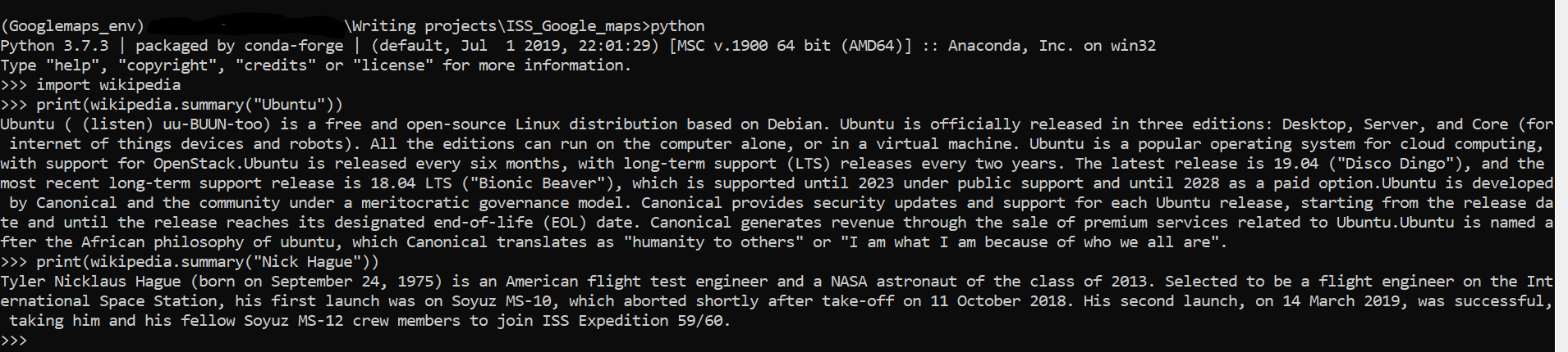
To start we need to install the Wikipedia API package. As I'm using the anaconda suite I used conda install. You can still use pip install. I’ve never used this package before I'm using this article to help me.
To test how the package worked, I opened up the console to run some function. Tried the example from the article above and my own example using the astronauts printed from earlier.
Now in the program, we need to way to feed the names into the Wikipedia function. So first we need to make a list of the names printed out earlier. This can be done by modifying the existing for loop to append the names to an empty list.
List_of_names = []

for person in astronauts_in_space:
    print(person['name'])
    List_of_names.append(person['name'])
['Alexey Ovchinin', 'Nick Hague', 'Christina Koch', 'Alexander Skvortsov', 'Luca Parmitano', 'Andrew Morgan']
Now we have the list of the astronauts' names we can then focus on coding up the Wikipedia function.
Using the code below is a for loop which iterates through the list of names we made earlier, prints a Wikipedia summary for the given value it has iterated through.
for every_person in List_of_names:
    print('-------------------------' * 3, end='\n')
    print(wikipedia.summary(every_person))
As we can see it is doing well but on the last name it threw an error:
wikipedia.exceptions.DisambiguationError: "Andrew Morgan" may refer to:
Andrew R. Morgan
Andrew Morgan (musician)
Andrew D. Morgan
Andrew Price Morgan
Andrew Morgan (cross-country skier)
Andrew Morgan (director)
This error happens when they are many articles under the same name. For now, I think I will hardcode a solution. As trying futureproof these type of error may be a bit difficult. To fix the issue I’ve added extra if statements in the for loop. So if it matches the string it will get the summary of the astronaut’s precise search.
for every_person in List_of_names:
    print('-------------------------' * 3, end='\n')

    if every_person == 'Andrew Morgan':
        every_person = 'Andrew R. Morgan'


    if every_person == 'Alexander Skvortsov':
        print('IF STATEMENT' * 5)
        every_person = 'Aleksandr Skvortsov (cosmonaut)'


    print(wikipedia.summary(every_person))
We can see the printed statements below:

Now I have the information about the cosmonauts. I want to move on to making the website.
I want to make the web interface with the flask library. As it lightweight and the website should not have too many features. When looking around I found that GitHub project that worked made dealing with flask and GoogleMaps easier. The project called Flask Google Maps the project made creating a template and a view for flask simpler. This is done by generating a google maps page with a flask template or using the package’s functions on a view to generate a map.
I opted to use the view method as its more clearer how to use.
@app.route("/")
def mapview():
    # creating a map in the view
    mymap = Map(
        identifier="view-side",
        lat=latitudefloat,
        lng=-longitudefloat,
        markers=[(latitudefloat, -longitudefloat)]
    )

    return render_template('home.html', mymap=mymap)
The code was based on the example code given in the readme. The longitude and latitude variables were imported from the previous script.
from main import longitudefloat, latitudefloat
This was the simple HTML page got:

The map was able to pin the location of the ISS and also have a simple heading. But later on, I noticed that generating a new map was not needed as I already generated one using my previous script. So decided to replace this newly generated map with my old one.
This was done by replacing the mapview function with only a pass statement. Which would only return the google maps HTML file.
def mapview():
    pass
    return render_template('my_map.html')
But the big issue popped out when the marker was not showing. After a few hours trying to fix the issue I found that i should just use my custom template based on the official google JavaScript API page for adding markers example code.
So now my webview function looks like this:
def mapview():
    latitude = latitudefloat
    longitude = longitudefloat
    return render_template('From_google.html', latitude=latitude, longitude=longitude)
The only code I’ve changed in the HTML file are the numbers defining location of the map to flask variables for the template. Later I change the code so it does say the location is Uluru. This was simple done to test out the code quickly without breaking the whole file.
function initMap() {
  // The location of Uluru
  var uluru = {lat: , lng: ;
  // The map, centered at Uluru
  var map = new google.maps.Map(
      document.getElementById('map'), {zoom: 4, center: uluru});
  // The marker, positioned at Uluru
var marker = new google.maps.Marker({position: uluru, map: map});
When running the flask local server this is the result:

This I would say it’s even better than the previous versions of the map. Mainly because the marker looks more modern.
Now the next steps are to develop the mini-biography sections below the map.
Google maps and ISS location with python
This new project involves the use of two APIs, google maps and open notify (ISS location). The goal of the project to collect real time data of the international space station’s location then be able to pin that location on google maps. I got the idea from this website. But the difference is they pinned it on there on map system.
To start we need to get the API get delivers the ISS data. The API returns a JSON file containing the latitude and longitude of the ISS along with a timestamp. First I tried to use the examples used in on the open notify website which is the API I would be using.
Which looked like this:
import urllib2
import json

req = urllib2.Request("http://api.open-notify.org/iss-now.json")
response = urllib2.urlopen(req)

obj = json.loads(response.read())

print obj['timestamp']
print obj['iss_position']['latitude'], obj['data']['iss_position']['latitude']

# Example prints:
#   1364795862
#   -47.36999493 151.738540034
But the code when I was trying to run was outdated. As this example of code is python 2. And even fixing the syntax errors trying to get the urlib2 library to run correctly was a bit difficult. The solution was to use a third-party library called requests. Which makes dealing with HTTP requests stupidly easy.
To get the JSON file using the requests library I only had to do this:
import requests

r = requests.get('http://api.open-notify.org/iss-now.json')
print(r.json())
And the print statement below:

As we can see the requests library made stuff a lot simpler. Now next task is to print the useful information from the JSON file above. Using the code from the website I mentioned in the beginning of the post. I will extract the longitude and latitude of the ISS.
The code used is below:
result = r.json()

location = result['iss_position']
latitude = location ['latitude']
longitude = location ['longitude']

print('latitude:', latitude)
print('longitude:', longitude)
Printed statements below:

Now we able to extract the latitude and longitude from the JSON file. Now we need to start getting the google maps API ready so we can input this data in.
I created an separate environment before I installed the google maps library for python. After I installed the library I went to the google cloud platform to fetch an API key so I can use the program. Used the example code on the library README file, Tested the google maps one of functions out. It was able to print out this JSON file.

So I just need to replace the example coordinates with my own. So replaced the numbers with the latitude and longitude variables.
Example code

reverse_geocode_result = gmaps.reverse_geocode((40.714224, -73.961452))

my code
reverse_geocode_result = gmaps.reverse_geocode((latitude, longitude))
The replacement worked and it returned this file JSON file.

As we can see in the file the ISS is flying over the Atlantic Ocean at the of running this code. But data is not too useful for are project as we want to plot coordinates over a map. To find the solution I was googling around. Then found the package gmplot which should the trick. The package genrates a html file containing javascript to allow users plot there data on google maps.
So I imported the new gmplots package. Based on the code on the README file. I placeed the map in the area which is based on the latutude and longitude variables.
google_maplot = gmplot.GoogleMapPlotter(latitude, longitude, 13)Next is the API key for the gmplot package. I used the same API key for the gmap package. Next is to make the marker plot location of the ISS.
google_maplot.apikey = [API_KEY_HERE TypeError: must be real number, not str ]

hidden_gem_lat, hidden_gem_lon = latitudefloat, longitudefloat
google_maplot.marker(hidden_gem_lat, hidden_gem_lon, 'cornflowerblue')
The reason why latitudefloat and longitudefloat exists is because when I was running the orginal latitude and longtuitade varibles. The google_maplot.marker fucntion threw this error:
TypeError: must be real number, not strMade new variables that turned the variables into floats.
latitudefloat = float(latitude)
longitudefloat = float(longitude)
After that I ran the program I opened the got error saying the map cant be loaded. The page said check the web console for the error message. The error I got is ApiNotActivatedMapError So I had to activate another api for map to load. The API was the Maps JavaScript API.
Now fixing that issue I was able to load the location of ISS. So it gave an general area. But the marker does not appear. Found the solution when googling around. Found a solution on the one of the issue pages on GitHub. I needed to go into the package itself to change the code.
From this:
self.coloricon = os.path.join(os.path.dirname(__file__), 'markers/%s.png')

to this:
self.coloricon = 'file:///' + os.path.dirname(__file__).replace('\\', '/') + '/markers/%s.png'
The most likely reason why the code was failing is that windows dealing with slashes(escape characters) a bit differently. So the windows probably did not open the markers file correctly.
After running the program again we get this result (I’ve zoomed out quite a lot see the location relative to other places in the earth. ):

Now the goal of the project is now fulfilled, as we can now run the program get the location of the ISS on the map. But I think more features can be added to the program later on like a web interface or giving information which astronauts are in the ISS at the given moment.
You can find the code on Github:
https://github.com/tobiolabode/ISS_Google_maps